VLSI Korea
Before adding ADC bits, has the input voltage settled?
SAR ADC accuracy is determined across the signal path. Acquisition time, channel switching, the input filter and amplifier dynamics need a shared timing and error budget.


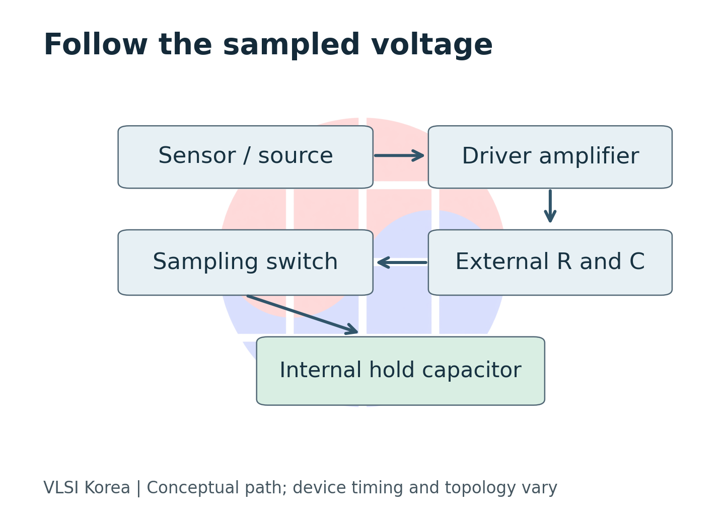
A slowly changing sensor can still demand a fast transient response at the ADC input. When the sampling switch closes, the voltage on the sampling capacitor must be restored. Choosing a resolution and then comparing amplifier MHz is not sufficient. The decisive question is how much error remains when the sample is committed. The board designer chooses the input filter and driver; the firmware designer chooses acquisition time and channel order. Both decisions need to refer to the same waveform.
VLSI Korea view: The design unit for precision conversion is the entire signal path up to the instant the input enters its allowed error band.
Why a slow sensor can need a fast input circuit
SAR means successive approximation register. The sampling SAR ADCs discussed here distinguish acquiring an input from converting the held voltage into a digital code. Microchip identifies source output impedance, the internal switch and the hold capacitor as contributors to acquisition requirements. It also distinguishes conversion time from acquisition time. Any overlapping phases or additional preparation intervals must be checked in the specific device data sheet. Microchip acquisition-time guide
A slowly moving sensor therefore does not establish that a slow input transient response is acceptable. Charge from the previous sample, charge left by internal conversion and the next channel voltage can differ. Even a temporarily flat waveform at the external input pin does not prove that the internal hold capacitor has reached the same value. Define the observation point before comparing a measurement with a model.
| Interval or node | What it means | Design question |
|---|---|---|
| Acquisition | Input is being captured | Has the internal sample settled? |
| Conversion | Held value is digitized | When can acquisition resume? |
| Input pin | External observation point | Does it represent the internal node? |
| Sample boundary | Voltage is committed | Is residual error within budget? |
Analog design automation makes this distinction newly relevant. The ATLAS preprint, submitted on 2026-10-07, investigates transistor sizing under multiple performance constraints. Only its abstract and submission history were checked for this article; it is not cited as an ADC measurement or production validation. Our editorial interpretation is that research can expand the methods used to find circuit candidates without choosing the system timing conditions against which those candidates must be judged. ATLAS abstract and history
Another bit changes the required waiting time
A useful starting point is a single-time-constant model. For initial voltage difference ΔV, time constant τ and elapsed time t, residual magnitude is |e(t)| = |ΔV| exp(−t/τ). With input span VFS and resolution N, ideal code spacing is VFS/2^N. Allocate a separate settling limit ε and the required wait becomes t ≥ τ ln(|ΔV|/ε). If the initial error is already below the limit, a negative result is not a waiting time. This has the same form as the RC approach in Microchip AN4225. The numbers below are our calculations under explicit assumptions, not device specifications. AN4225 acquisition analysis
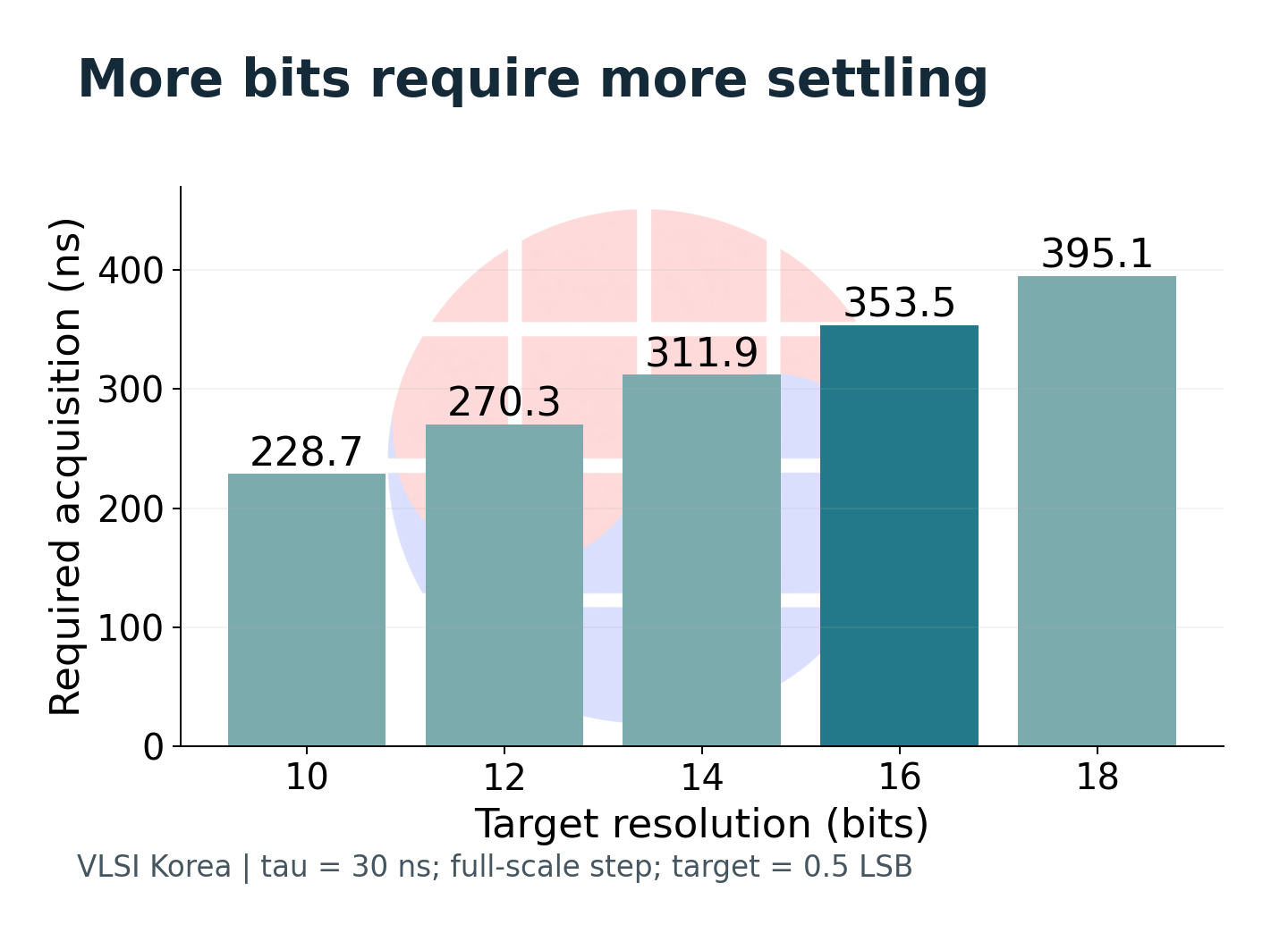
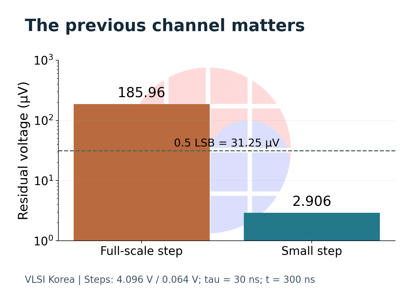
Assume a 4.096 V input span, a 16-bit target and τ = 30 ns. Code spacing is 62.5 µV; allocating 0.5 LSB to settling gives a 31.25 µV limit. Following a full-scale step, waiting 300 ns leaves approximately 185.96 µV, or 2.975 LSB. Producing a valid output code does not mean that this error has disappeared. The same model requires approximately 353.5 ns.
| Assumed quantity | Value | Interpretation |
|---|---|---|
| Input range | 4.096 V | Full-scale step also assumed |
| Resolution | 16 bits | Ideal code spacing: 62.5 µV |
| Time constant | 30 ns | Single-pole model parameter |
| Available acquisition | 300 ns | Residual: 185.96 µV / 2.975 LSB |
| Settling target | 0.5 LSB | Required time: 353.5 ns |
The immediate design choice is concrete. Retain the same signal path and acquisition must grow; retain the same window and the initial step or effective time constant must shrink. Reducing the resolution to pass the calculation also changes the measurement requirement. Confusing the converter's stated resolution with the accuracy actually required can produce a mathematically correct calculation and an incorrect system decision.
Channel switching puts the filter's roles in conflict
Consecutive samples on one channel may differ little. A multiplexed circuit instead connects sensors at different voltages in sequence. In the same model, an initial difference of 0.064 V leaves approximately 2.906 µV after 300 ns, far below the full-scale transition result. Repeated measurements of one channel cannot establish accuracy for every scan sequence. Verification needs the combinations and transition directions that approach the allowed range limits.
An external capacitor can provide some of the charge demanded at switching, while the input filter limits broadband noise. Larger capacitance and resistance can also lengthen recovery. ADI's front-end design article describes this compromise among noise, settling and stability. An amplifier's small-signal bandwidth does not independently guarantee large-step settling or stability with a capacitive load. ADI front-end amplifier and RC design
| Change | Potential benefit | What must be checked |
|---|---|---|
| Larger reservoir capacitor | Smaller immediate voltage disturbance | Recovery and driver stability |
| Higher series resistance | Isolation from capacitive load | Settling and distortion |
| Longer acquisition | More time to recover | Throughput and latency |
| Smaller channel-to-channel step | Lower initial error | Worst-case signal ordering |
Experiments with component values should separate possible causes. Changing only the resistor is different from changing both resistance and capacitance. An improvement after reordering channels can suggest memory of the preceding channel, but does not establish the mechanism by itself. Source impedance, switch charge and amplifier recovery may interact. Calculations narrow the candidates; circuit-specific waveforms and codes distinguish among them.
Half an LSB does not erase every other error
Allocating 0.5 LSB to settling is not a guarantee of total accuracy. Reference error, gain and offset, nonlinearity, noise and settling residue have different characteristics. Deciding which terms require a worst-case sum and which can be combined statistically requires evidence about signs, correlations and distributions. Applying a root-sum-square operation to every term can conceal systematic errors linked to channel transitions.
VLSI Korea view: The allowed settling error is an allocation from the system error budget, not a number automatically supplied by ADC resolution.
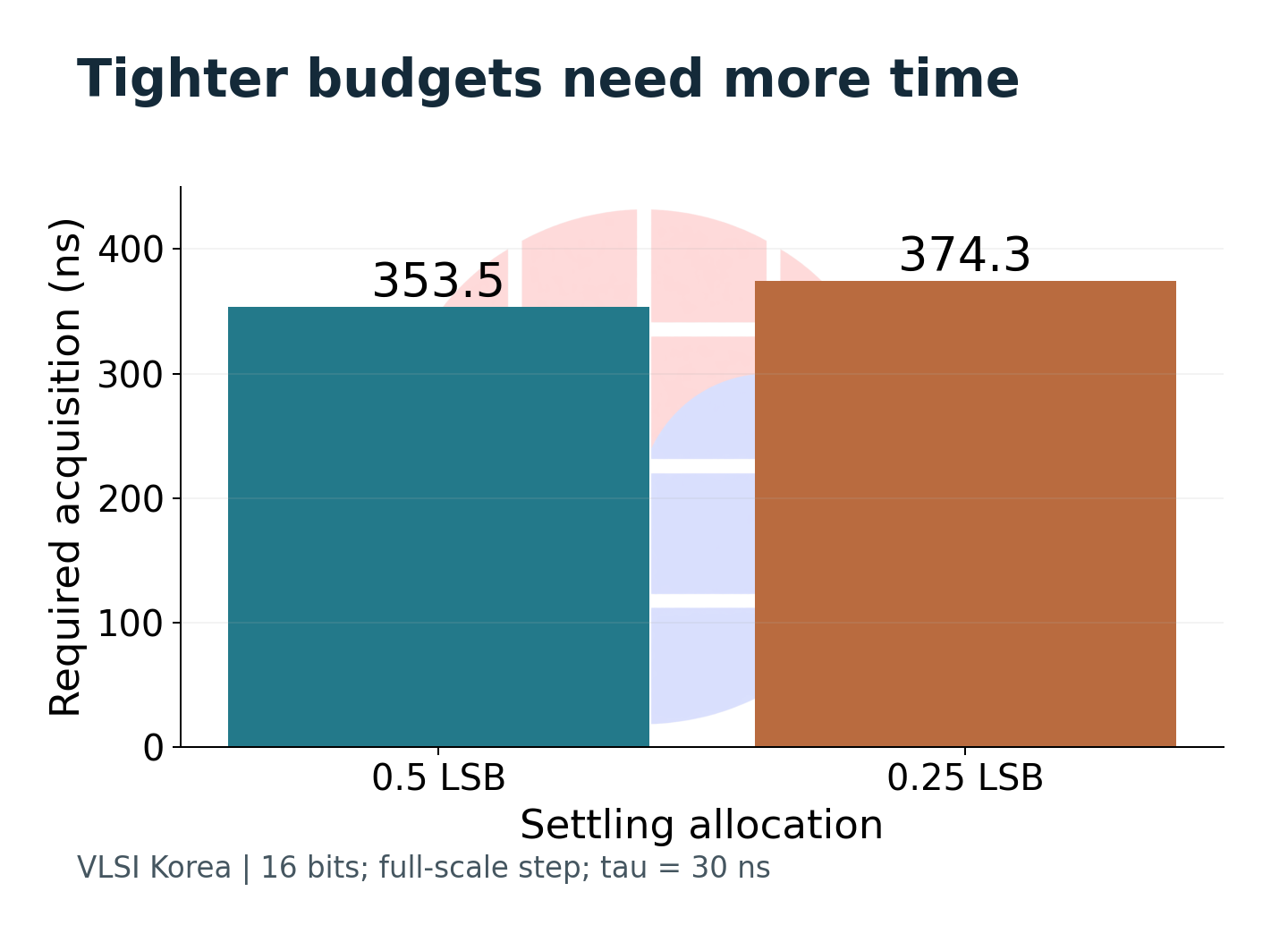
Reducing the example's settling allocation to 0.25 LSB gives a 15.625 µV limit and extends the required wait to approximately 374.3 ns. That does not prove that the other errors fit the remainder. Define total error for the measurement task before allocating its components. Absolute voltage accuracy, repeatability and signal-to-noise ratio are distinct requirements and should be documented as such.
| Error class | Useful observation | Do not assume |
|---|---|---|
| Settling residue | Code versus acquisition delay | Random, independent noise |
| Gain or reference error | Response across input range | Removed by longer acquisition |
| Offset | Response near a known level | Improved by more output bits |
| Noise | Distribution under fixed conditions | Equivalent to channel memory |
Nor is the single-time-constant approximation a guaranteed model of the entire input circuit. TI SBAA173A analyzes a second-order response with the external RC network, internal sampling switch and hold capacitor together. Even that analysis begins with an ideal-voltage-source amplifier assumption. The chart's τ therefore cannot simply be replaced by the external resistance-capacitance product for every circuit. If an internal node is slower, or the amplifier rings, the model must be reconciled with the observed response. TI SBAA173A equivalent circuit and assumptions
An architecture can return time, with conditions
Buying a faster amplifier is not the only system-level response. Changing when an ADC reconnects its input, or how it handles internal charge, changes the burden on the external circuit. ADI describes a long acquisition phase and a high-Z mode in the AD4000/AD4003 family, with high-Z reducing nonlinear charge disturbance. The same document says to disable high-Z for multiplexed inputs. A feature useful for a slow single input is not automatically suitable for scanning channels. These are manufacturer explanations, not independent measurements made for this article. ADI architecture explanation
The multiplexed example CN0385 shows switching to the next channel shortly after conversion starts to provide settling time. Distinguish the next channel reaching the external node from recovery after the internal sampling capacitor reconnects. Moving the channel-switching instant does not hide every part of settling behind conversion. A reproducible comparison has to preserve the circuit's actual timing and operating mode. ADI CN0385 multiplexed-input settling
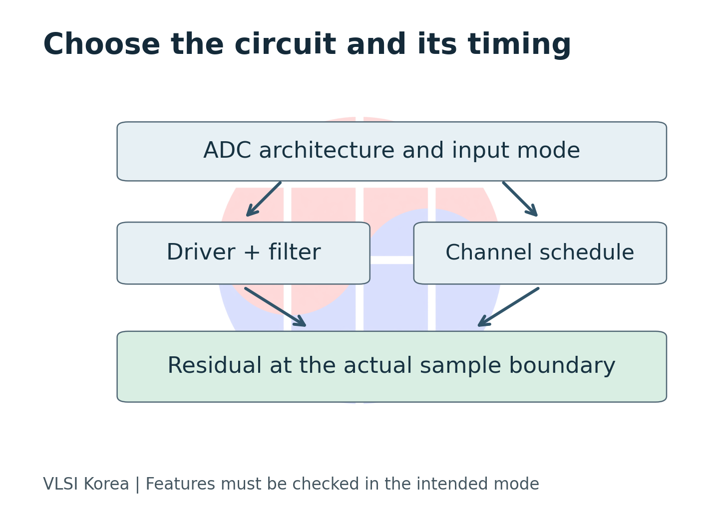
| Design owner | Decision | Evidence needed |
|---|---|---|
| Board designer | Driver and input filter | Stability, swing, residual at sampling |
| Firmware designer | Acquisition and channel order | Actual timing and worst-case sequence |
| Converter supplier | Input mode and architecture | Mode-specific limits and timing |
| System validation | Acceptable measurement error | Budget, test conditions and margin |
This division also helps interpret supplier literature. Microchip's MCU guidance provides a starting point for source impedance and acquisition settings. TI's equivalent-circuit analysis establishes limits of a simple model. ADI's front-end documents and circuit example connect external drive to internal operation. These are evidence for different design questions, not results to add together as one benchmark. The photographed OPA627 provides historical physical context for an operational amplifier; it is not claimed to be a suitable driver for these examples.
What Korean measurement and test teams can change first
For teams designing semiconductor test boards or industrial sensor modules in Korea, the first useful change is not a component ranking. Including acquisition settings and channel order in circuit verification can help preserve reproducible conditions across analog and firmware teams. This is an application proposal, not an observation that a named Korean company encountered the issue or achieved cost savings. A stronger driver may add power, area and thermal burden; a longer wait changes throughput and latency. Compare these costs for the actual board and operating mode.
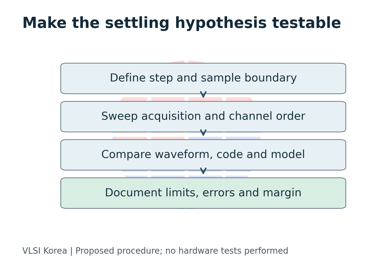
Start by alternating channels close to the ends of the input range. Vary acquisition time and observe the direction and magnitude of code movement. Compare against a fixed-channel result to isolate transition dependence. Record supply, temperature, gain and input range, and check the loading added by the measurement probe. Where the internal node cannot be observed directly, an external waveform alone is insufficient for acceptance: code changes and model predictions should agree as well.
| Test | Expected evidence | Interpretation limit |
|---|---|---|
| Sweep acquisition delay | Residual trend versus time | Other errors may dominate late |
| Alternate distant channels | Dependence on prior channel | Does not isolate every mechanism |
| Repeat one fixed channel | Baseline distribution | Does not validate multiplexing |
| Vary allowed operating conditions | Margin across required range | Tested range only |
There is a falsifier. If the error remains unchanged after acquisition is extended sufficiently and is independent of the preceding channel, settling becomes a weaker explanation. Revisit the reference, leakage, calibration, grounding and measurement error. Conversely, if waiting helps but the response does not follow a single exponential, expand the model. Choosing the correct explanation comes before obtaining an attractive plot.
Over the next 6–12 months, watch for condition-specific evidence about features that ease input drive, rather than nominal ADC resolution alone. The next review date is 2027-04-09. Look for newly published multiplexing restrictions, acquisition timing, models including actual loads and reproducible waveforms. Analog design automation can also be evaluated on whether these conditions enter its objectives and verification. The conclusion is practical: before adding bits, obtain evidence that the system has captured the voltage correctly.
Sources
- Microchip: ADC Acquisition Time: marked updated 2023-11-09. Acquisition versus conversion time.
- Microchip AN4225 / DS00004225A: 2021, RC approximation and buffer limitations.
- TI SBAA173A: revised 2010-11, input equivalent circuit and ideal-amplifier assumption.
- ADI: Front-End Amplifier and RC Filter Design: technical background on filtering and drive conditions.
- ADI: Next-Generation SAR ADC: AD4000/AD4003 features and mode restrictions. Historical technical material, not a new announcement.
- ADI CN0385: switching timing and settling in a multiplexed example.
- ATLAS, arXiv:2610.10985v1: preprint submitted 2026-10-07. Abstract and history only; no claim of acceptance or silicon validation.
Disclosure
VLSI Korea prepared this explanatory contribution from public technical documents and preprint metadata. AI assisted research, drafting and translation. Calculations and diagrams are original work under stated assumptions, not measurements, SPICE validation or product recommendations. Manufacturer explanations are distinguished from editorial interpretation. The photograph is used under ZeptoBars' reuse permission with attribution.