VLSI Korea
Thermal resistance is not a chip constant: why junction-temperature estimates fail
Datasheet thermal resistance, package surface temperature and average power answer different questions. Match the board boundary conditions and heating timescale before using the result to make a design decision.


Multiply chip power by datasheet thermal resistance and add ambient temperature: the arithmetic looks straightforward. But if the test board and cooling conditions differ from the product, the answer changes. Measuring a surface or switching the load briefly changes the required inputs again. The useful question is what must be checked before a thermal-resistance calculation becomes a prediction for an actual product?
VLSI Korea view: The first choice in thermal design is the boundary condition that matches the temperature being estimated, rather than the smallest resistance in a table.
A number that includes the escape path
Junction temperature refers to the semiconductor's active region. Ambient air, the package top and the board are different observation points. At steady state, junction-to-ambient thermal resistance RθJA is the junction-to-ambient temperature difference divided by device power dissipation. Its unit is °C/W, equivalent to K/W for a temperature difference. TI describes it as strongly dependent on system conditions. It should therefore not be read as a material constant that survives any board change. TI thermal-metric guide
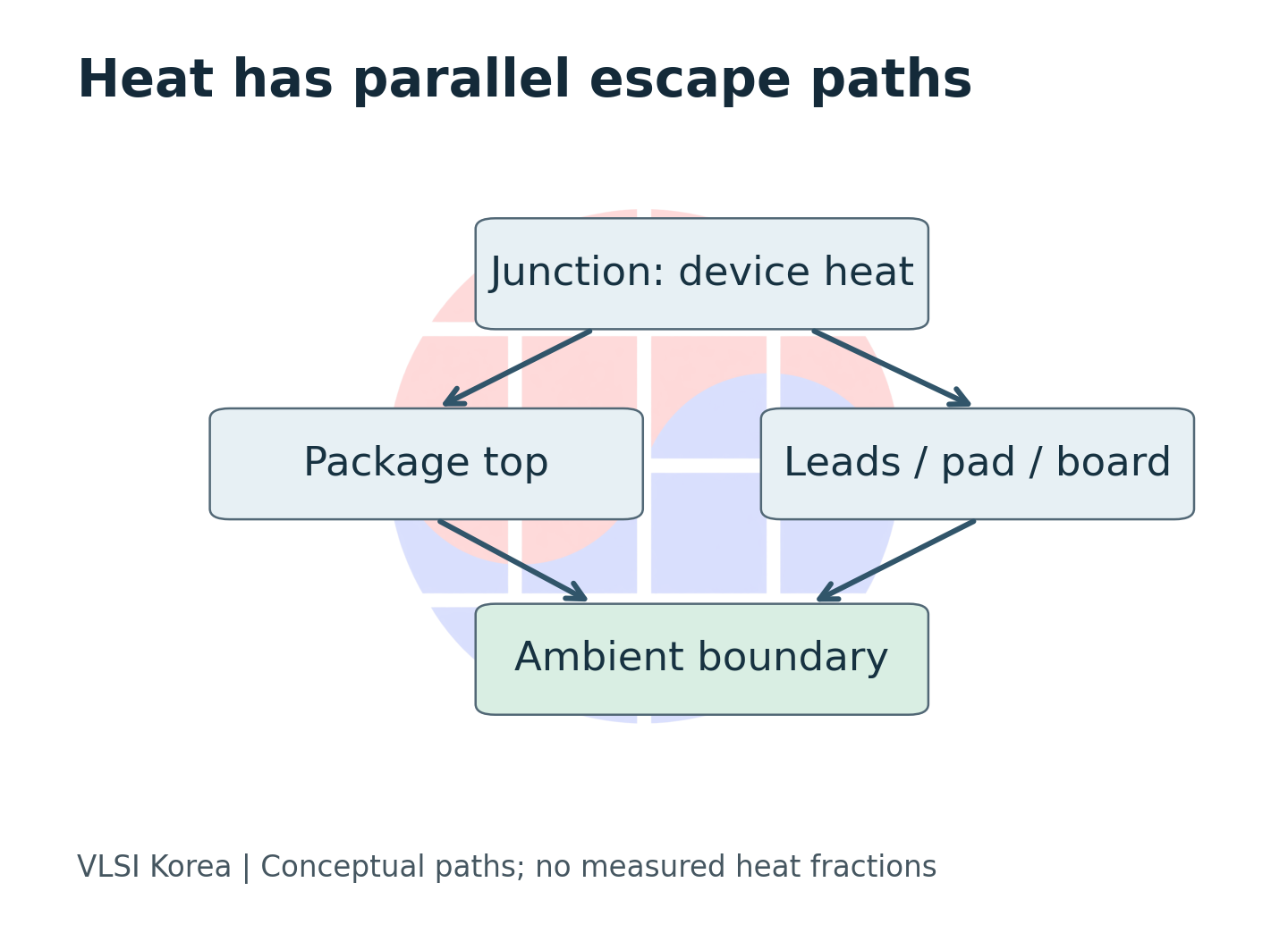
Heat divides among the package top, leads, exposed pad and board. More board copper changes an external escape path without changing the mechanism generating heat in the die. A neighboring component can also warm the board into which the chip rejects heat. Substituting laboratory air temperature for ambient temperature inside the product is then a separate assumption. The location of the ambient measurement belongs in the input record.
| Input | What must match | Failure if omitted |
|---|---|---|
| Power | Heat dissipated in the device | Load power counted as device heat |
| Reference temperature | Ambient, top or board location | A metric paired with the wrong sensor |
| Boundary | Copper, vias, airflow and enclosure | Test-board result treated as universal |
| Time | Steady state or specified waveform | Average substituted for peak |
A component-selection engineer needs comparable datasheet conditions. An engineer debugging an existing board needs to infer an internal temperature from an accessible measurement. The former chooses a package and board arrangement; the latter decides whether to restrict load or redesign. Those decisions require different starting points even when the same table is open. Reading TI's metric guide, Nexperia's boundary-condition study and ADI's thermal-design tutorial together makes that distinction useful. Nexperia boundary-condition study · ADI thermal-design basics
The same regulator, a different copper area
A linear regulator dissipates power inside the device because of the difference between input and output voltage. TI's LM1117 datasheet provides a thermal-design procedure and test results for different copper areas. The selected rows below cover SOT-223, no bottom copper, and a tab attached to top copper. This historical design example illustrates how an external heat path changes the temperature even when the device name stays the same. LM1117 thermal-design table
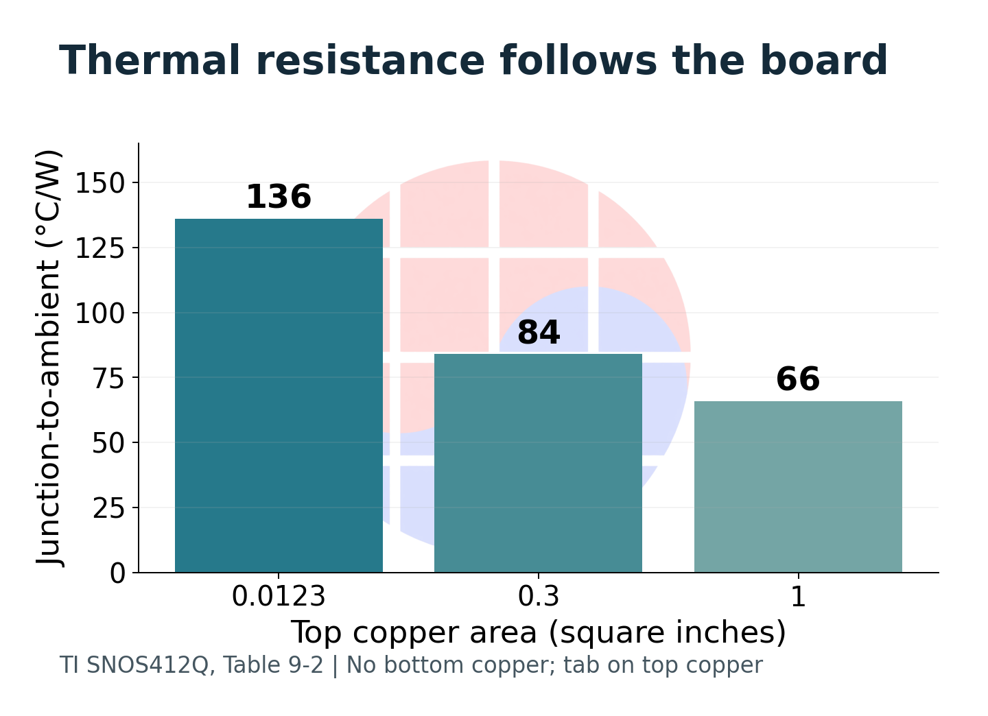
The resistance column comes from the manufacturer's tests; the temperature columns are this article's calculations. They assume constant device loss of 0.5 W and ambient temperature of 40 °C. These are not temperatures measured on an actual LM1117 board. The photograph is also contextual: ZeptoBars identifies the historical die as an LM1117, but the photo does not establish its manufacturer or package variant. It is not presented as TI's test specimen.
| Top copper area (square inches) | RθJA (°C/W), TI test | Rise at assumed 0.5 W (°C) | Junction at assumed 40 °C ambient (°C) |
|---|---|---|---|
| 0.0123 | 136 | 68 | 108 |
| 0.3 | 84 | 42 | 82 |
| 1 | 66 | 33 | 73 |
The designer has changed the space available for heat spreading, not the part number. There is no general law that resistance keeps falling in proportion to added copper area. Another path can become the bottleneck, reducing the value of additional copper. Connecting points in a table does not create a guaranteed curve for an arbitrary board. The comparison needs the complete structure, including geometry, copper thickness, connections and airflow.
The power input needs its own check. Counting all delivered output power as device heat exaggerates cooling demand. Omitting quiescent or other losses can make the margin optimistic. Before replacing a package, establish actual dissipation and ask whether a board change addresses the problem. Our editorial implication is to compare component cost together with board area and verification work.
A surface reading requires the right denominator
A hot package top is useful evidence, but its temperature is not junction temperature. RθJC and ΨJT are easy to confuse here. RθJC corresponds to a test boundary that directs heat toward a specified case surface. ΨJT divides the junction-to-top temperature difference by total device power dissipation. It does not assert that all that heat crossed the top surface. Despite sharing a unit, it is not a pure path thermal resistance. Definitions of RθJC and ΨJT
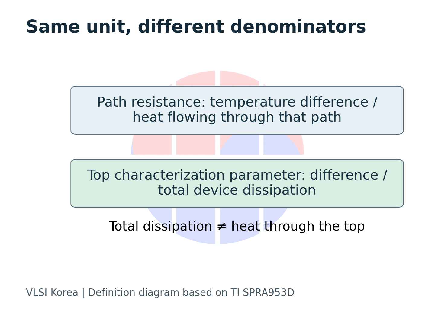
Assume that ΨJT characterized under conditions sufficiently similar to the board is 2 °C/W. A measured top temperature of 70 °C and dissipation of 2 W imply an estimated junction temperature of 74 °C. Incorrectly substituting RθJC of 10 °C/W from a different test gives 90 °C. The difference of 16 °C comes from changing the denominator and boundary conditions, rather than a suddenly hotter chip. These values are assumptions explaining metric confusion, not specifications of a particular product.
| Assumed input or result | Value |
|---|---|
| Measured top temperature | 70 °C |
| Device loss | 2 W |
| Applicable ΨJT | 2 °C/W |
| Estimated junction | 74 °C |
| Misapplied RθJC | 10 °C/W |
| Incorrect estimate | 90 °C |
ΨJT is not a universal correction for any surface reading either. A top-mounted heat sink changes the heat partition and therefore the characterization conditions. Sensor-induced cooling and infrared emissivity errors remain. TI distinguishes heat-sink applications from the use of ΨJT and calls for the relevant heat path instead. Recording the observation point, sensor attachment and surrounding structure preserves the meaning of the calculation. Surface measurement and heat-sink scope
Short heating needs a time response
Steady-state thermal resistance describes a sufficiently long heating interval. During a short load, the device and its surroundings store heat, so the temperature does not immediately reach the steady-state value for the same power. A transient thermal impedance or validated dynamic model is needed to describe time response. ADI's steady-state relationship is a starting point, not a universal peak-temperature calculation for every pulse duration. Steady-state temperature-rise relationship
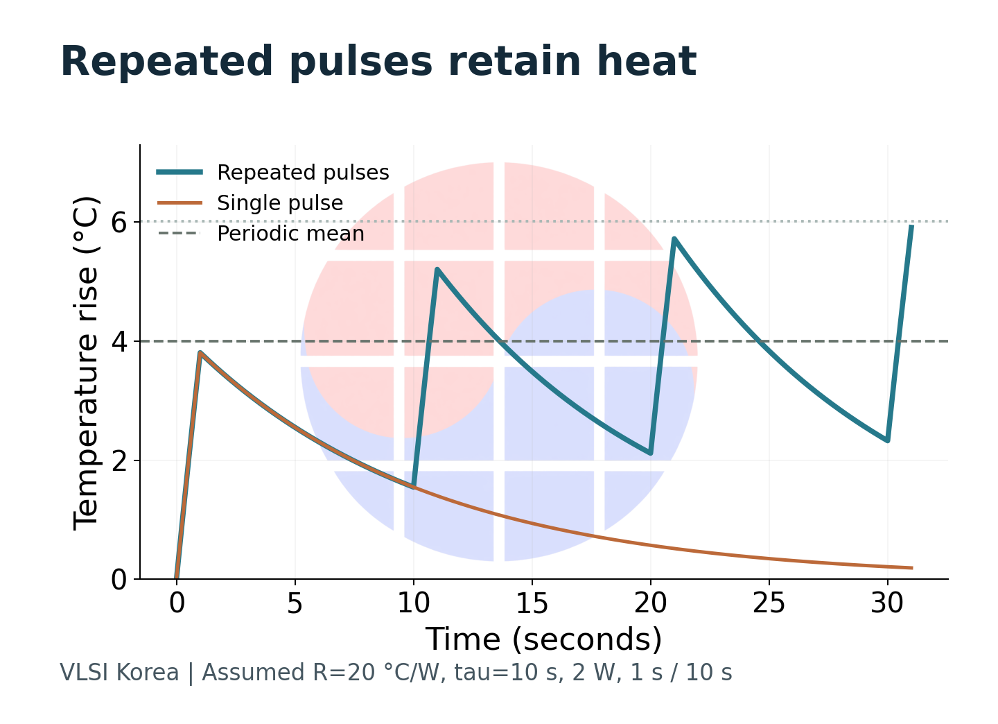
To expose the distinction, construct a linear model with a single thermal capacitance. Assume resistance R of 20 °C/W, time constant τ of 10 s and on-state loss P of 2 W. With fixed ambient, the temperature rise ΔT obeys τ·dΔT/dt + ΔT = P·R. A single pulse starting at ambient gives ΔT(t) = P·R·[1 − exp(−t/τ)]. This is an explanatory calculation, not a fitted model of a real chip.
| Assumed waveform | Temperature-rise result (°C) | Meaning |
|---|---|---|
| Continuous 2 W | 40 | Steady state |
| One 1 s pulse from ambient | 3.81 | End of first pulse |
| 1 s on, 10 s period, repeated | 6.02 | Periodic steady-state peak |
| Same repeated waveform | 4 | Periodic mean |
During repeated pulses, cooling in the off interval leaves residual heat for the next pulse. The peak above is P·R·[1 − exp(−t_on/τ)] / [1 − exp(−T/τ)], where T is the period. The mean rise obtained from average power is below the peak, and the first pulse ends below the eventual periodic peak. Decimal places describe calculation output, not claimed measurement precision.
Boundary condition: Equal average power does not establish equal peak junction temperature.
A real package has multiple time constants, and dissipation can vary with temperature. Do not copy the assumed time constant into a product model. Check whether a model explains both the heating and cooling intervals of the actual load and stays within the required error after sustained repetition. If it does not, use relevant transient data or a validated thermal model.
Ask about the model before narrowing the error bar
Recent thermal-metrology work also addresses uncertainty explicitly. The arXiv manuscript by Chen, Wang and Jiang was submitted on 2026-10-06. It describes physics-based variable transformations for uncertainty in coupled parameters extracted from multilayer thermoreflectance. Our reading here is limited to the abstract and metadata. That does not establish better junction-temperature prediction for a particular product, or validation in manufacturing measurements. Thermoreflectance uncertainty abstract
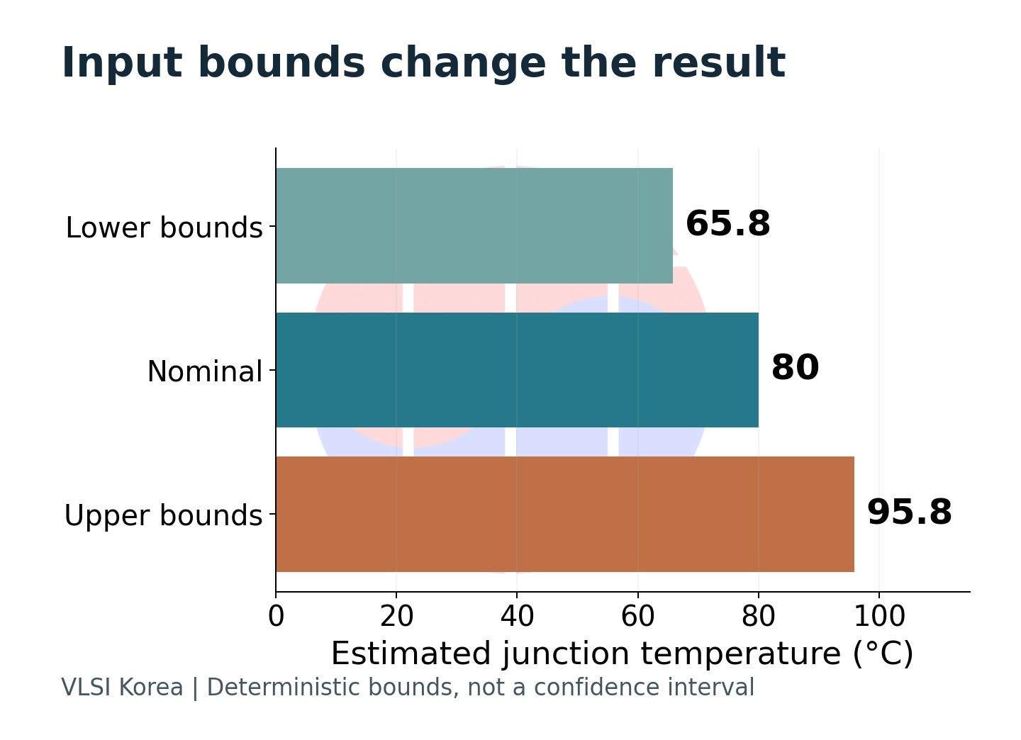
Our practical example is a simpler input-bound calculation. Assume independently variable bounds of 2 ± 0.2 W dissipation, 20 ± 4 °C/W effective resistance and 40 ± 3 °C ambient. The steady-state equation gives a nominal 80 °C, but combining the extreme inputs spans 65.8–95.8 °C. Without probability distributions this is not a confidence interval. It is separate from the preceding pulse calculation.
| Case | Ambient (°C) | Loss (W) | Effective resistance (°C/W) | Junction estimate (°C) |
|---|---|---|---|---|
| Lower input bounds | 37 | 1.8 | 16 | 65.8 |
| Nominal inputs | 40 | 2 | 20 | 80 |
| Upper input bounds | 43 | 2.2 | 24 | 95.8 |
More precise arithmetic is not the main issue. Without evidence that the product's effective resistance lies inside the assumed bounds, a tidy interval can legitimize the wrong model. If loss and cooling vary together with temperature, the independent-bound assumption also needs review. Measurement scatter, sensor error and model-structure error should not disappear into one small error bar.
Order the checks around the claim. A surface-based estimate needs the observation point and applicable correction; package selection needs comparable boards and cooling; a pulse peak needs time response. A result becomes useful at design review when the engineer can explain which changed input would reverse the decision, not merely display more decimal places.
Evidence to carry into the next board revision
When Korean fabless, packaging and board-design teams divide this work, the handoff should extend beyond a part number to the experimental conditions. The package thermal model, copper and via structure, and circuit loss waveform must describe the same use case. Otherwise, each team's calculation can be internally correct while the assembled product's temperature remains unexplained. This is our collaboration proposal, not a measured failure rate for the Korean industry.
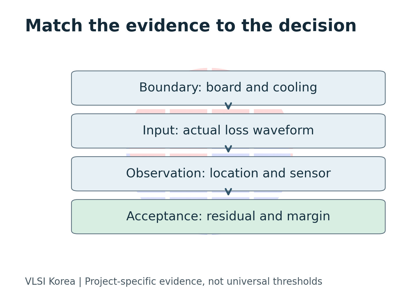
For the next prototype, choose representative loads and retain both dissipation waveforms and temperature observation points. Controlled cooling changes and repeated-load tests can help distinguish explanations. The model should be reproducible from the recorded inputs, with residuals traceable to board conditions, loss, sensing or dynamics. If junction temperature cannot be observed directly, retain that limitation. Agreement with a surface temperature alone does not validate the internal hotspot.
| Reader decision | Evidence to request | What would change the decision |
|---|---|---|
| Keep the package | Matched board and cooling comparison | Required margin absent after board changes |
| Increase allowed load | Loss waveform and periodic temperature | Peak exceeds project limit or uncertainty budget |
| Trust a surface estimate | Sensor placement and applicable metric | Cooling path changes the heat partition |
| Accept a compact model | Residuals across representative conditions | Errors persist outside the fitted condition |
Over the next 6–12 months, watch how reproducibly component and package suppliers deliver models with explicit conditions, rather than just competing on the lowest resistance. Set the next review at 2027-04. Look for public evidence that jointly exposes transient-model error, reproducibility after board changes and measurement uncertainty. This is not a forecast of any company's product release.
There is a clear condition that would overturn the need for further model complexity. If validation covering the product's board, cooling, loss, observation point and time behavior repeatedly meets the project's error allowance and temperature margin with a simple resistance calculation, keep that simplicity. Every design does not need a complicated model. But that conclusion must come from matched measurement and comparison, not from the component table alone.
Disclosure
This educational article synthesizes public technical documents and a research abstract. Calculations and diagrams are original VLSI Korea work under explicit assumptions, not product test results. The real photograph carries source and reuse information. AI assisted drafting and translation. The article does not guarantee a product's allowable temperature, lifetime or manufacturing quality.
Sources
- Texas Instruments, Semiconductor and IC Package Thermal Metrics, SPRA953D, revised 2024-03.
- Texas Instruments, LM1117 datasheet, SNOS412Q, revised 2023-01, Table 9-2 and thermal design section.
- Nexperia, IAN50019, Thermal boundary condition study on MOSFET packages and PCB substrates.
- Analog Devices, MT-093, Thermal Design Basics, Rev.0, 2009-01.
- Chen, Wang and Jiang, arXiv:2610.09192v1, submitted 2026-10-06. Abstract and metadata only; journal-reference field is not independent publication verification.
- ZeptoBars, historical LM1117 die photograph, 2012-11-15, CC BY 3.0.