Wafer Inspection Sampling: Miss Probability and Containment Delay

Inspecting more wafers and missing fewer defects are different claims, connected by a model. In a lot of 25 wafers containing 2 affected wafers, a uniform random sample of 3 still has a 77% probability of missing both. This is a finite-population calculation with perfect detection, not an observed fab result.

VLSI Korea view: Approve a sampling plan against separate population, spatial-selection, detection and containment-delay requirements.

Wafer inspection sampling is the rule that selects some lots, wafers, dies or inspection regions for observation. Its scope differs from classifying an image the instrument has already acquired, and from assuring the defect level of finished shipments.

1. Put the denominator back into inspection coverage

Process engineers have two jobs here: decide which excursions limited inspection capacity must detect, and determine where and when production must stop after detection. This article supports the choice of sample count and location, and the choice between expanding inspection and shortening feedback.

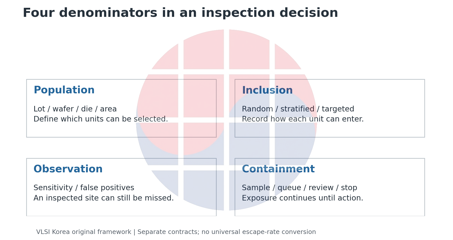
First freeze the sampling unit. The fraction of lots selected, the fraction of wafers inspected within those lots, and the area observed on a wafer have different denominators. A more accurate image classifier does not directly observe defects on a wafer excluded upstream.

We call this the population, selection, observation and containment framework. Define the universe that can be inspected, record the rule by which units enter the sample, then attach the conditions for detecting an affected unit and the time required to contain production.

NIST/SEMATECH distinguishes lot acceptance from estimating lot quality. A “sample pass” alone therefore does not identify the population or the risk being constrained.

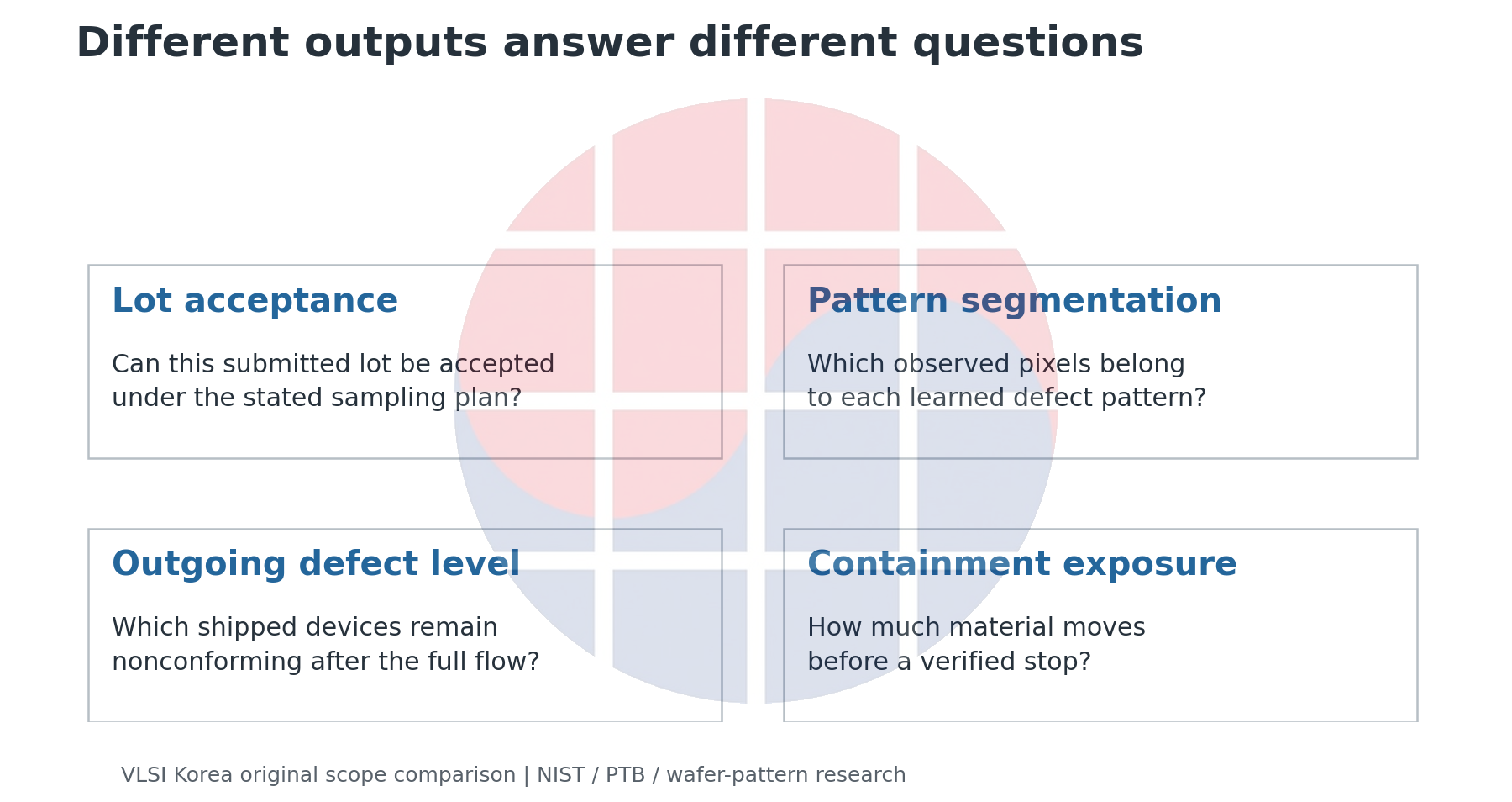
For final-test fault coverage and outgoing defect level, start with the existing yield, binning and defect-level analysis. The probabilities here are not converted into that defect level. An electrically failing die and a particle that signals a process excursion are different events.

Why revisit this boundary now? SePArate, publicly posted on 2026-08-31, separates pixel-level defect patterns using image-level labels. As interpretation of observed data improves, the operational temptation is to extend that confidence to unobserved space and time. That warning is VLSI Korea's inference, not a performance claim made by the paper.

2. What does inspecting 3 of 25 wafers miss?

Fix the population at N=25 wafers, with K=2 affected wafers. Select n uniformly without replacement and assume every selected affected wafer is detected. A miss means that the sample contains no affected wafer.

There are C(N,n) possible samples and C(N−K,n) entirely unaffected samples. Thus P(miss)=C(N−K,n)/C(N,n). C denotes the number of combinations; the numerator is 0 when the sample exceeds the unaffected population. This does not imply that K is known in a real lot. It asks how vulnerable a plan is to a specified hypothetical excursion.

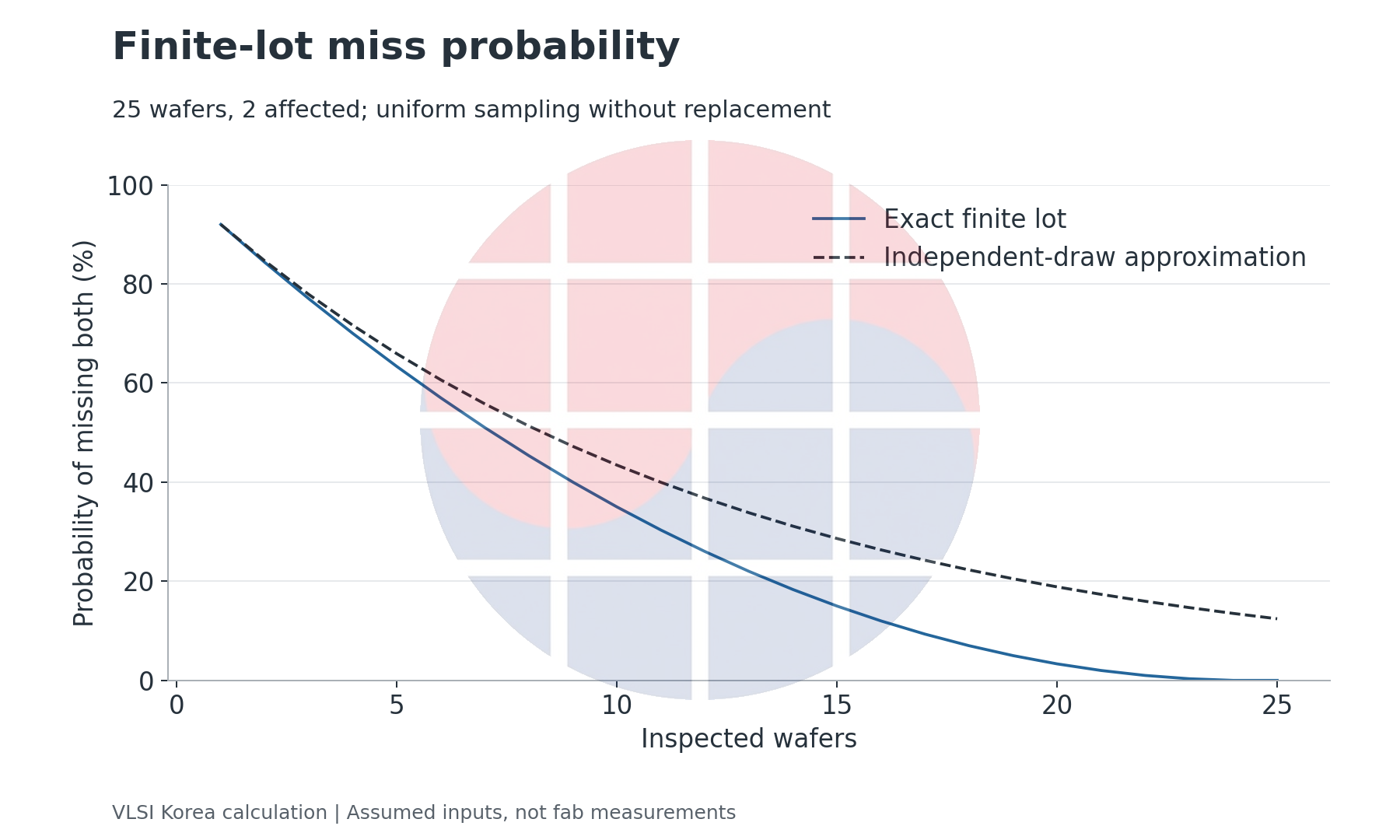
The results are 77% for n=3, 63.33% for n=5 and 35% for n=10. More samples reduce this particular miss probability, but the calculation does not establish that a small sample is sufficient. The requirement must specify the excursion size and tolerated miss probability, rather than merely record how many wafers were inspected.

The independent-draw approximation, (1−K/N)^n, also diverges from the exact finite-lot answer. Each unaffected wafer removed from a finite lot reduces the unaffected population remaining. Treating every draw as having the same probability becomes harder to justify as the sampling fraction increases.

NIST's operating-characteristic curve depends on both n and the acceptance number c. The any-detection example here corresponds to the simple c=0 condition. A plan that accepts some detected affected units requires a different calculation.

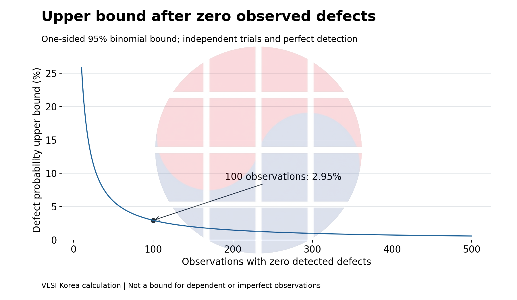
An entirely clean sample answers another question again. With independent Bernoulli observations and perfect detection, 0 findings in 100 observations give a one-sided 95% upper bound of 1−0.05^(1/100), approximately 2.95%. Observing 0 defects does not prove a population defect fraction of 0. Nor should this bound be attached unchanged to spatially dependent samples.

3. A sampled defect can still go undetected

Now switch models. Each site independently has defect probability p=0.01, and the conditional sensitivity for detecting a defective inspected site is s=0.8. Assume no false positives on good sites and an alarm whenever any detection occurs.

The probability of a detection at one site is ps, so the probability of no detections in n sites is (1−ps)^n. This is an unconditional zero-detection probability under an independent population with a specified p. It is neither conditional acceptance risk for a bad lot nor the posterior probability that a lot is good after a pass.

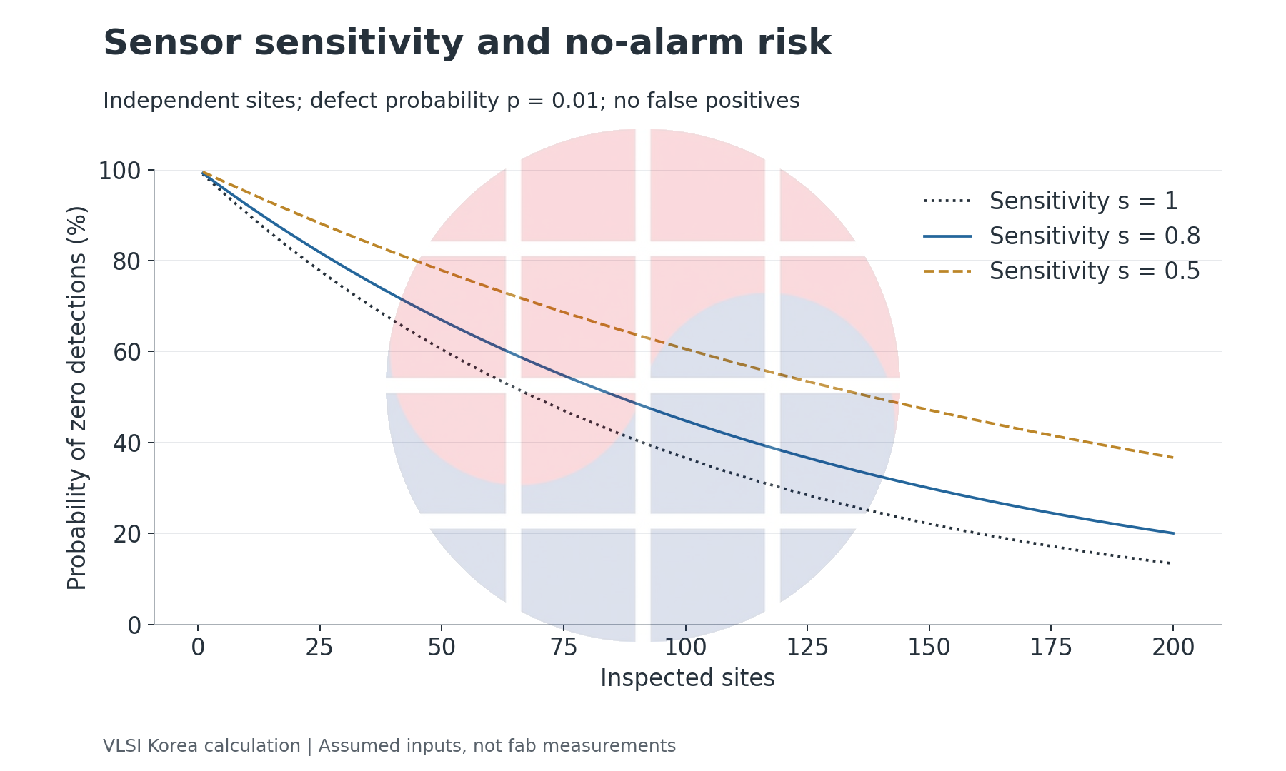
At n=50, 100 and 200, this probability is 66.92%, 44.79% and 20.06%, respectively. At least 373 observations are required to bring it to 5% or below under these assumptions. That count is not a ready-made inspection recipe: the definitions of p and s, spatial independence and repeatability of the observation conditions must be established first.

A brochure accuracy number cannot substitute for s. Sensitivity must be checked for the defect class, size, observation conditions and threshold used in the decision. Without independent ground truth for missed defects, sensitivity remains unknown. Counting what the instrument found does not reveal everything it failed to find.

There is also a cost on the other side. Suppose each good site independently has false-positive probability q=0.001. When every site is good, the probability of at least one false alarm is 1−(1−q)^n. At n=50, 100 and 200, the results are 4.88%, 9.52% and 18.14%.

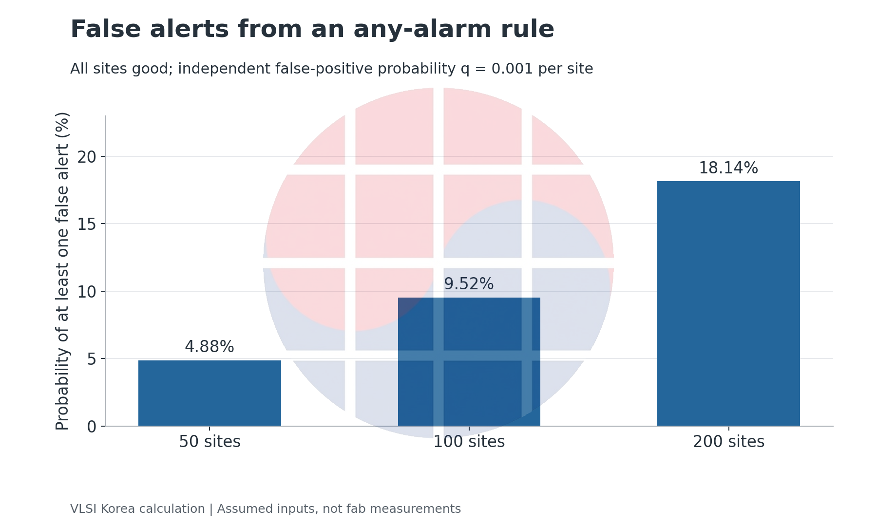
This is not an argument against larger samples. It means that an any-alarm policy needs review capacity and a confirmation rule alongside its sample count. Unnecessary holds can enlarge the inspection queue and delay confirmation of a real excursion. We model the timing consequence separately below.

TU Dresden's distribution-analysis research separates defect detection from incorrectly rejecting good chips, and distinguishes prediction of backend status from frontend observation. Its results do not supply a transferable fab-specific s or q. Moving performance between labels and process stages requires separate validation.

4. The same 10 observations can carry different information

To isolate spatial dependence, construct a 10×10 grid instead of a physical wafer shape. Exactly one row, comprising 10 of the 100 cells, is affected, and detection is perfect. Every strategy inspects 10 cells. The illustration is not a reconstruction of a measured wafer defect map.

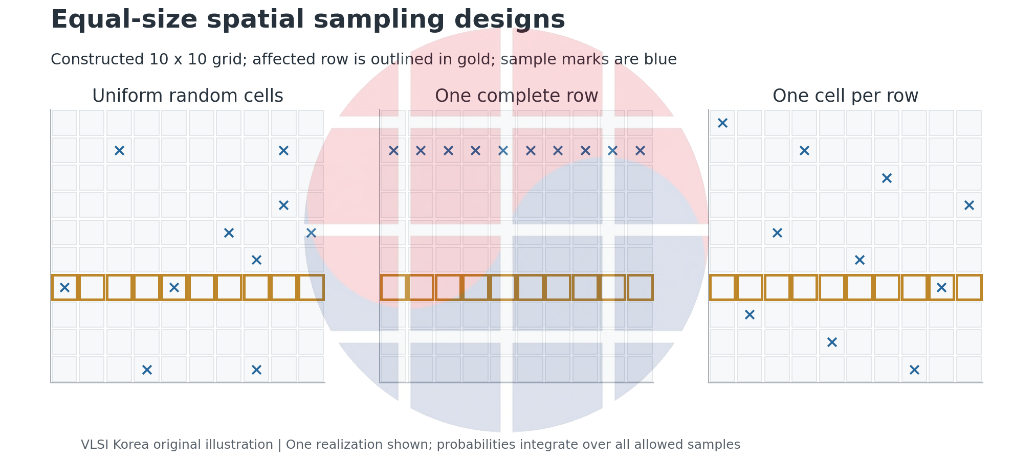
Selecting 10 cells uniformly without replacement gives miss probability C(90,10)/C(100,10), approximately 33.05%. Selecting one complete row uniformly gives 90%, the probability of avoiding the affected row. Selecting one cell uniformly at random within each row, independently across rows, gives 0% in this particular example.

Every cell has the same marginal inclusion probability, 0.1, under all three strategies. What changes is which cells are selected together. Reading one entire row concentrates observations in a shared local environment; sampling across rows breaks that dependence. Equal coverage does not imply equal information.

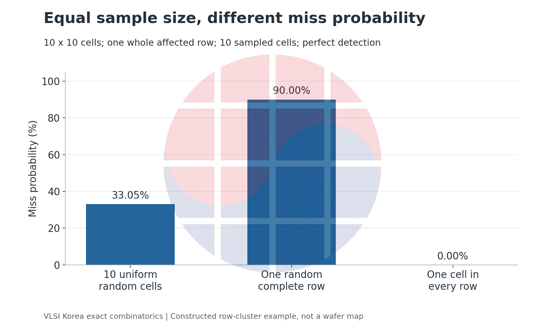
Stratification is not universally optimal. The 0% result requires an entirely affected row and perfect detection. A small local cluster, an oblique scratch or a pattern between selected locations changes the answer. Without a defensible geometry model, a design optimized for one toy pattern is incomplete.

A practical plan may need strata for chamber, lot order, wafer slot and time as well as wafer coordinates. More strata leave fewer observations in each. The plan should state the representativeness claimed with the available sample budget and the coverage it does not provide.

The Politecnico di Milano team's open-set wafer-monitoring research distinguishes known-pattern classification from novelty detection in observed defect coordinates. Our operational inference is that recognizing familiar patterns and finding new excursions need different validation. Future lots and changed recipes belong in separate evaluation partitions.

5. A classifier score is not inspection coverage

SePArate separates overlapping patterns into pixel masks. Its MATDefects data use DRAM-mat bits, while MixedWM38 uses wafer-level dies. Identical-looking binary pixels therefore have different physical denominators. The authors' published examples below are not inputs to our sampling experiment.

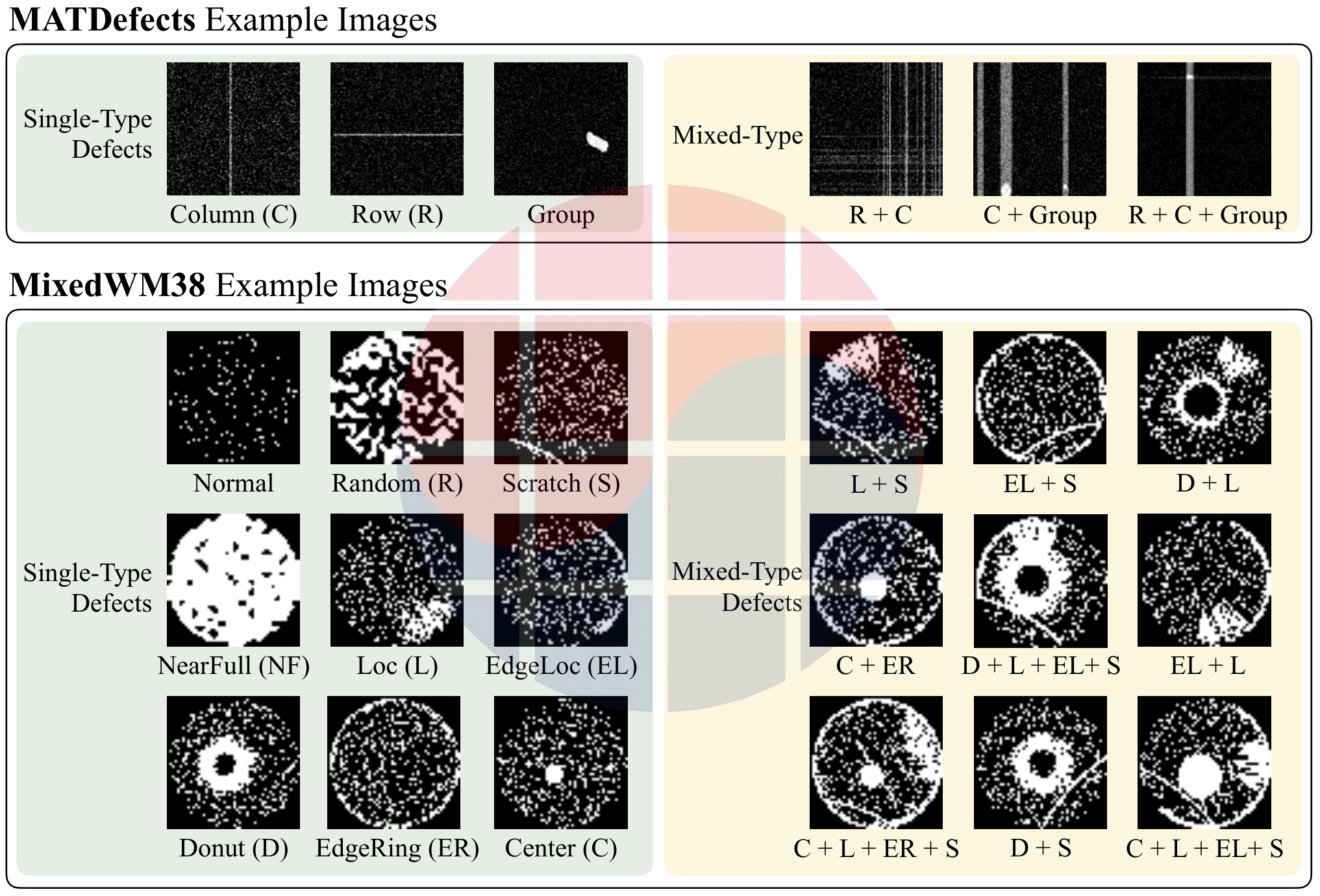
This distinction changes the acceptance criterion for an analysis algorithm. If a model separates patterns among already observed defective locations, evaluate mask quality and the downstream decisions it improves. The score does not establish that unmeasured wafers are unaffected.

SePArate connects encoder training, spatial knowledge transfer and training on synthetic mixed-defect data. The following source figure explains the authors' synthetic-data generation; it is not raw metrology. See the public paper for the method.

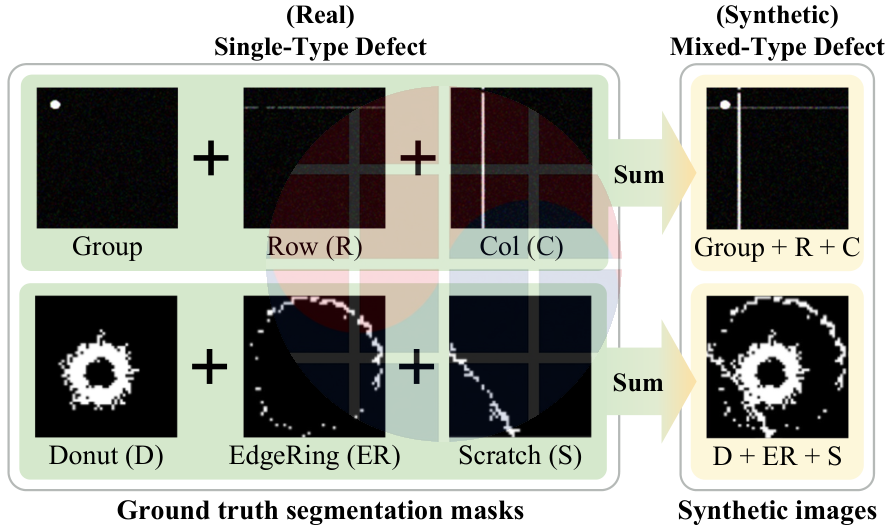
Our proposed qualification experiment is independent of the model's name. Hold observation selection fixed while comparing classifiers, then hold the classifier fixed while comparing selection policies. Changing both at once makes it harder to identify the cause of an improvement or a newly introduced blind spot.

Performance on a random training split does not promise performance in future production. Add evaluations separated by time, equipment and recipe changes, and retain a route for reviewing unfamiliar patterns. Whether synthetic patterns represent actual excursion frequency and geometry is another independent question. We do not claim fab deployment or yield improvement for the paper.

6. Late containment increases the material exposed

Adequate selection and detection still leave the containment clock. In this model, a persistent excursion is detected at the next inspection with certainty. Let Δ be the inspection interval, d the delay from the inspection instant through results, review and interlock, and r a constant production rate.

If excursion onset is uniform within an inspection interval, mean exposure is r(Δ/2+d), with a worst-phase bound of r(Δ+d). Use consistent time units. This model excludes repeated inspection misses, batch movements, reentrant flows and variable queues.

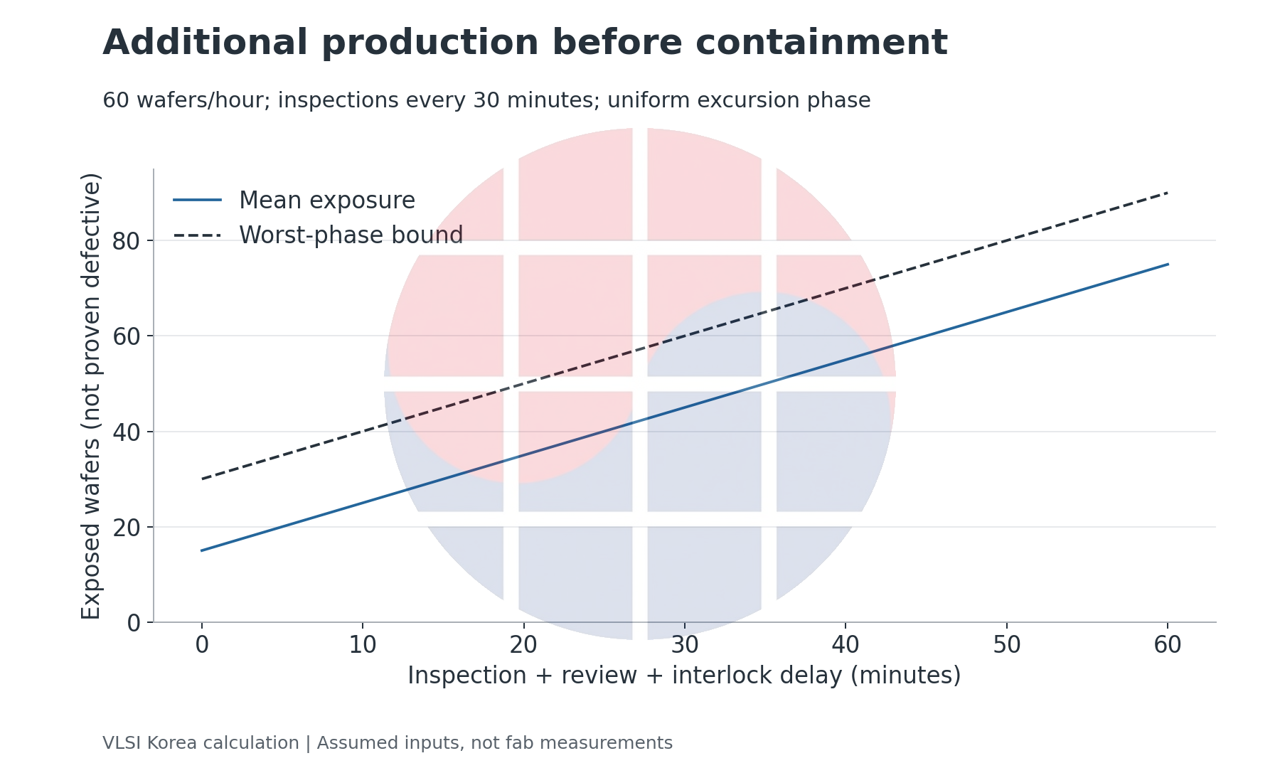
Set r=60 wafers/hour and Δ=30 minutes. With d=5 minutes, mean exposure is 20 wafers; with d=45 minutes, it is 60. The same inspection interval therefore leaves 40 additional wafers exposed because feedback is slower. Those wafers are not all proven defective or destined for scrap. The count describes material potentially requiring investigation and disposition.

Assume accumulated WIP value of $2,000 per wafer. The additional 40 wafers represent $80,000 of gross WIP exposure. This is not realized loss. Without recoverability, defect impact, downstream cost and disposition evidence, we do not convert it into revenue, margin or free cash flow. The number identifies the additional inputs a business decision needs.

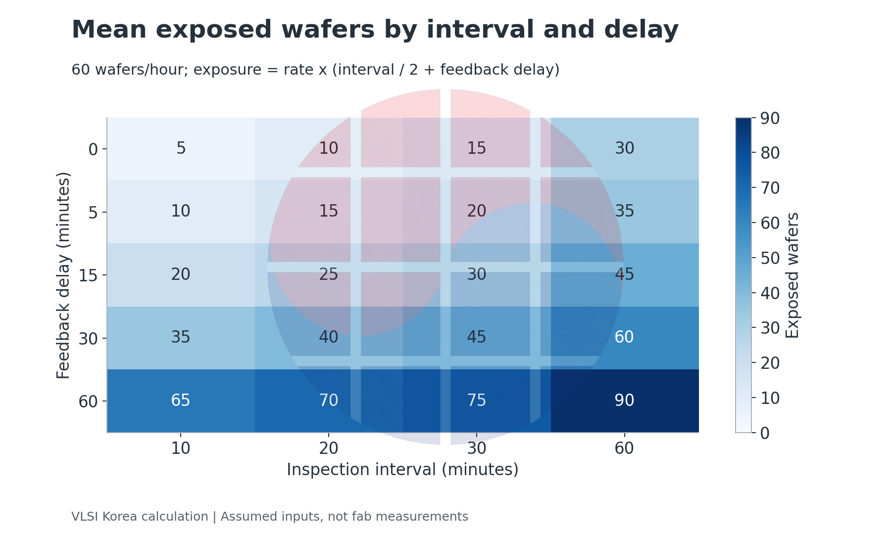
Under these conditions, reducing d can matter as much as increasing inspected coverage. Conversely, if excursions are rare and most holds are false alerts, added review congestion can offset the benefit of expanded inspection. Put sample completion, alarm creation, disposition and the actual stop of the relevant chamber on one time axis.

Do not rely only on the average. Occasional long waits produce tail exposure that a mean d cannot describe, and production rate may vary. Reconstruct the exposed material set from actual event timestamps and lot movements when those effects matter. A convenient model should not erase the flow it is supposed to inform.

7. A qualification checklist and conditions that reverse the conclusion

For Korean process, yield and inspection teams, the shared specification needs more detail than a coverage target. Agree on the excursion to detect and the definitions of an affected wafer and an affected die. If coordinate conventions and chamber histories disagree, the sample's claimed scope is already wrong.

Separate p from s. The former belongs to the assumed defect-population model; the latter describes observation conditional on a defect. A changed confidence threshold requires another review of false-alert burden. Apparently low defect prevalence does not establish low detector miss probability.

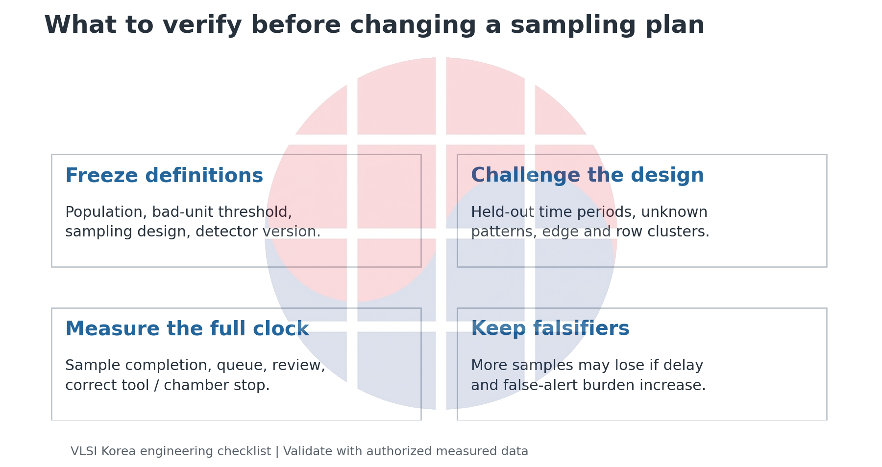
The working sequence is to freeze population and sampling rules, verify sensitivity against independent reference inspection, evaluate spatial and temporal holdouts, and verify feedback timestamps. The existing Yield Engineering workflow guide, in Korean, supplies organizational context. No proprietary production recipe or private fab dataset has been inserted into this analysis.

Destructive inspection adds another question: does the decision concern the original lot or the material remaining after the sample is consumed? A PTB-led preprint posted on 2025-08-07 addresses that distinction. It does not make the earlier combinatorial law incorrect; the event it describes can differ from the question about the remaining shipment.

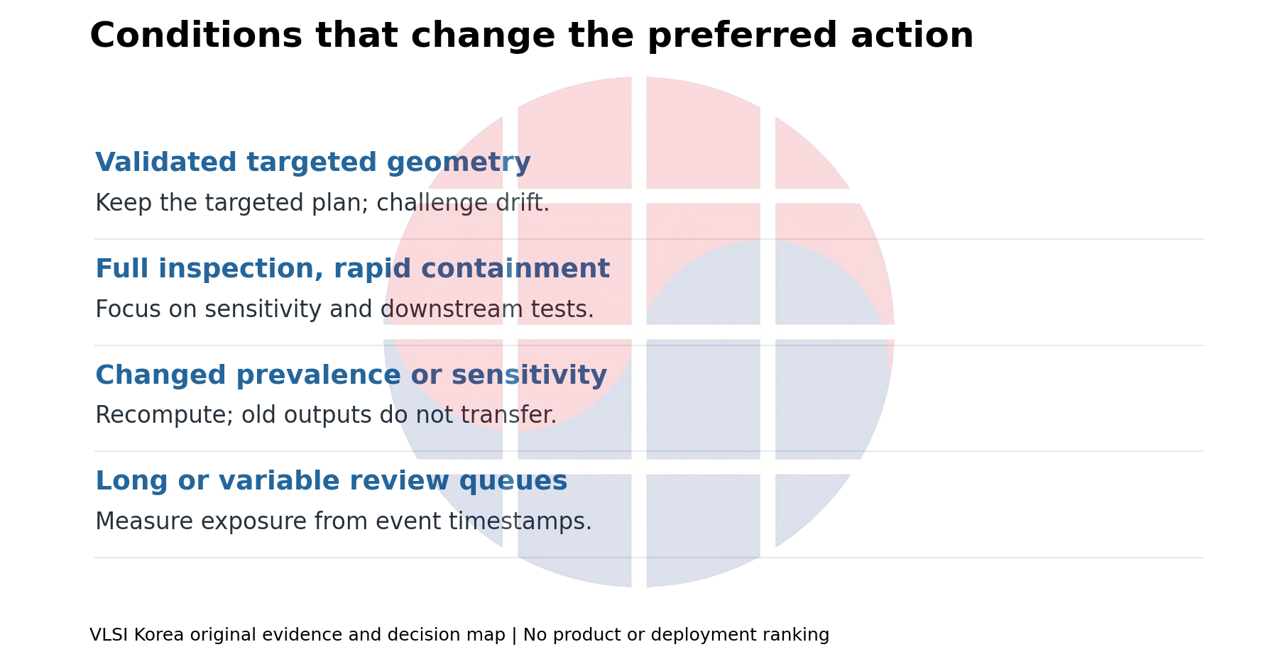
Boundary condition: Turning a sample with no detections into a pass for unobserved products requires a separate inference and validation.

The strongest counterargument is a production setting with a well-qualified targeted strategy. Inspecting a narrow region can be much more efficient than random sampling for a known defect geometry. Our toy comparison does not justify replacing that policy. Use it to design tests of whether the advantage survives new geometry or drift.

Another falsifier is full inspection with almost immediate containment. If sample selection and delay are no longer the dominant constraints, attention should move to sensitivity, classification or downstream testing. If p, s or spatial dependence differ from the assumptions, recompute the examples rather than preserving their outputs.

The following dates are editorial checkpoints, not product roadmaps: 2027-03-07 for defect-class sensitivity and spatial-holdout misses; 2027-06-07 for queue, review and interlock timestamps; and 2027-09-07 for unfamiliar patterns missed after recipe changes. They do not predict public data releases or improved results.

The object of approval is the bounded risk and its conditions, not the coverage number alone. Connect inclusion probabilities, detection conditions and actual containment timestamps before deciding whether to inspect more, change locations or shorten feedback.

Sources and method

Evidence checked: 2026-09-07. Models and inputs in this article are illustrative; no private fab data or measured deployment performance is asserted.

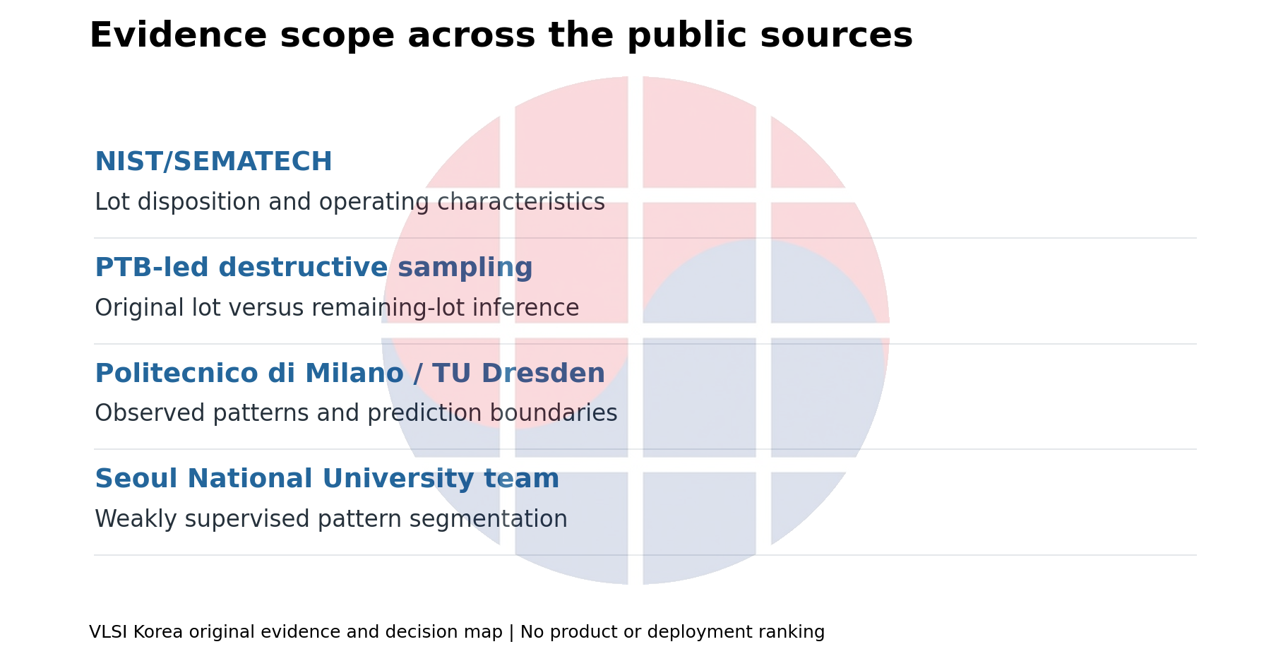
• What is Acceptance Sampling? (NIST/SEMATECH). Living handbook; page-specific publication date unavailable.
• Choosing a Sampling Plan with a given OC Curve (NIST/SEMATECH). Living handbook; page-specific publication date unavailable.
• Plans for acceptance sampling by attributes when observations are destructive (Physikalisch-Technische Bundesanstalt). 2025-08-07.
• Deep Open-Set Recognition for Silicon Wafer Production Monitoring (Politecnico di Milano). 2022-08-30.
• SePArate: Segmenting Patterns from Defects in Wafer Manufacturing Using Weak Supervision (Seoul National University). 2026-08-31.
• Defect Detection on Semiconductor Wafers by Distribution Analysis (Technische Universitat Dresden). 2021-11-05.

Source figures: Dain Kwon, Changmin Shin, Sunjong Park, Kanghyun Choi, Hyeyoon Lee, Jaewon Jang, Minseok Choi and Jinho Lee, SePArate. CC BY 4.0. Figures 2 and 5 reproduced from the public paper with a single VLSI Korea watermark added on 2026-09-07. No endorsement is implied.

AI-assisted research, calculations, translation and editing. VLSI Korea distinguishes cited findings from its own assumptions and interpretation.